TECHNICAL SYNTHESIS / LONG-CONTEXT SYSTEMS
BSH is a layout,
not a context limit.
Attention, memory, and what changes beyond 270,000 tokens
Klyff Harlley Toledo · October 23, 2026
Literature-based research note with original analytical illustrations. This is not a peer-reviewed paper or a hardware benchmark.
Abstract
Long-context language-model discussions often collapse three distinct questions: how tensors are arranged, how attention is computed, and what information persists between decoding steps. I separate these questions using explicit notation and a reproducible memory model. In the AWS Neuron documentation examined here, BSH denotes batch–sequence–hidden layout. It does not impose quadratic memory by itself. Dense pairwise attention has quadratic sequence arithmetic; a naive score allocation is quadratic, while tiled exact kernels avoid storing the full score matrix. Autoregressive KV-cache storage is linear in retained sequence length. Recurrent state-space and kernel-based linear-attention architectures change the computational representation, but a hybrid retaining global attention also retains context-dependent attention costs. An illustrative 270,000-token calculation exposes these differences without treating that length as a universal threshold. I conclude with a measurement protocol separating capacity, latency, precision, parallelism, and long-range task quality.
Keywords: BSH; tensor layout; prefill; decode; KV-cache; FlashAttention; Mamba-2; linear attention; hybrid models; long context.
1. Separate the layout from the algorithm
My starting point is a distinction: the location of numbers in memory is not the same thing as the mathematical interaction between those numbers. AWS documents BSH as (batch, sequence, hidden) and describes compiler opportunities such as reducing transposes and overlapping computation with collectives. It also discusses static-shape bucketing. These are implementation considerations, not a proof that BSH requires an S × S allocation. [1]
I use D for hidden width so that nq, the number of query heads, cannot be confused with the H in BSH. After projections, a query tensor may be logically viewed as B × nq × S × dh. The implementation may use another physical layout, tiling, packing, or sharding. Identical logical shapes can have different strides and communication costs.
| Symbol | Meaning | Illustrative value |
|---|---|---|
| B | Active sequences in a uniform-length batch | 1 |
| S | Retained sequence length | 270,000 tokens |
| D = nqdh | Hidden width in the simplified model | 4,096 |
| nq / nkv | Query heads / cached key-value heads | 32 / 8 |
| dh | Head width | 128 |
| L / La | Total layers / attention layers in the hybrid example | 32 / 3 |
| p | Bytes per stored element | 2 |
The dimensions above describe an explanatory configuration, not the undisclosed internals of a proprietary model. For uneven batches, each sequence contributes its own Sb; replacing them with one padded maximum can obscure substantial waste.
2. Where the quadratic term actually appears
For one attention head, the conventional expression is:
With a length-S prefill, the logical score matrix has S² entries per head. Counting each multiply-add as two floating-point operations, the two large attention products contribute approximately 4BnqS²dh operations per layer if treated as dense rectangular products. Causal masking can reduce the useful work by roughly a constant factor, but does not remove the quadratic sequence term. Projections, feedforward layers, normalization, softmax and communication contribute additional costs not captured by this term.
The original FlashAttention work shows how tiling and online normalization can compute exact attention without writing the full score matrix to HBM. The essential distinction is between logical pairwise interactions and simultaneously materialized intermediate storage. FlashAttention is not kernel-based linear attention. [2] FlashAttention-3 further targets Hopper execution through asynchronous overlap and low-precision techniques; its FP8 path also introduces numerical-precision considerations. None of these labels alone establish linear dense-attention arithmetic. [3]
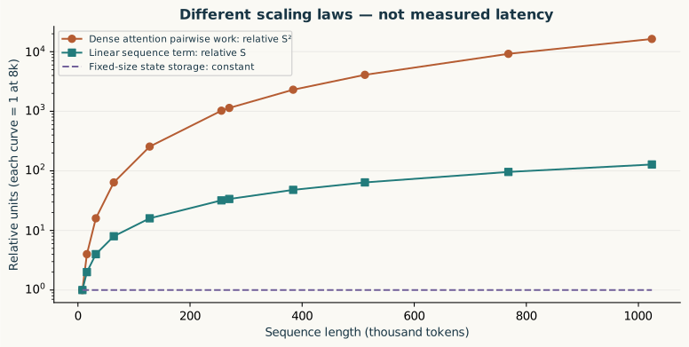
During decoding of a single new token, the query length is one while key length is S. The per-layer attention products therefore scale approximately as 4BnqSdh for that step. Generating T tokens while retaining the entire history accumulates work over S, S+1, …, S+T−1. “Linear per decode step” does not mean the total cost of an arbitrarily long generation remains linear in its final length.
3. A 270,000-token example without a mythical boundary
For a naive fully materialized score tensor, storage for one layer is:
The standard retained key and value tensors across L layers instead require:
The factor two represents keys and values. Grouped-query attention uses fewer KV heads than query heads, reducing the cache coefficient. It does not change linear dependence on retained S. [4] These equations exclude model weights, allocator fragmentation, runtime workspaces, quantization metadata, and temporary activations. They also assume uniform storage precision and uncompressed cache values.
Substituting Table 1 gives approximately 4,345 GiB (4.24 TiB) for the hypothetical 32-head score matrix in one layer, but 32.96 GiB for the entire 32-layer KV-cache. A single head’s naive score allocation would be about 135.79 GiB. These are deliberately different allocations; adding them as though a modern tiled kernel must store both would misrepresent its implementation.
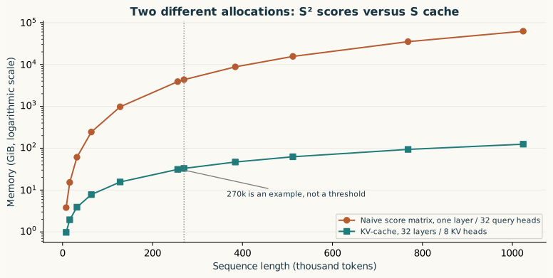
I use 270,000 solely because it motivates the question. None of the inspected sources establishes it as a universal physical or architectural limit. Available memory, model width, layers, precision, batching, kernel design, supported positions, sharding and task accuracy all matter. Doubling S quadruples the naive score term and doubles the cache term. There is no discontinuity at this particular token count.
Serving systems can redistribute cost without changing the underlying model. LoongServe investigates elastic sequence parallelism, adapting parallelism and KV movement across inference phases. That addresses deployment resource management; it is not evidence that layout alone changes attention’s asymptotic behavior. [5]
4. What changes when the sequence representation changes?
4.1 Blockwise exact attention
Blockwise Parallel Transformer combines blockwise attention computation with feedforward fusion to reduce memory pressure. Its contribution should be classified as an execution and intermediate-memory strategy, rather than automatically grouped with recurrent architectures that replace full history with a bounded state. [6] When benchmarking, the relevant comparison includes achieved arithmetic throughput, HBM traffic and peak allocation—not only the complexity class.
4.2 Kernel-based linear attention
Katharopoulos and colleagues express attention through feature maps and exploit associativity to permit linear-in-sequence processing at fixed feature dimensions. [7] A simplified causal formulation accumulates a matrix C and normalization vector z:
zt = zt−1 + φ(kt),
yt = φ(qt)ᵀCt / [φ(qt)ᵀzt].
Here, a feature dimension r gives a matrix state with r × dv entries per head. Fixed dimensions make its recurrent state independent of history length, but those dimensions still affect compute, capacity and numerical behavior. This is a different operator or representation; it should not be described as FlashAttention’s exact softmax implementation.
4.3 State-space models and compressed history
Mamba-2 develops structured state-space duality and efficient structured computations relating SSMs and attention. [8] A schematic recurrence is ht=Atht−1+Btxt, with an output derived from ht. This sketch communicates state updates, not a complete implementation. Fixed-shape recurrent inference state changes how history is carried forward; training can still allocate sequence-dependent activations and employ parallel algorithms.
My inference is that “no growing token cache” must not be equated with “perfect access to unlimited history.” With finite precision, a bounded state has finitely many possible configurations, whereas the number of possible token histories grows with length. Distinct histories must eventually share a state. The practical question is which distinctions remain useful for the task—not whether compression has made information constraints disappear.
4.4 Hybrids retain the cost of their attention layers
The Bamba report describes Bamba-9B with 29 Mamba-2 layers and three full-attention layers. Those layers use eight KV heads and 32 query heads. They are not described as sparse merely because there are fewer of them. The report also discusses context extension of the attention component. [9]
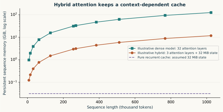
Under a simplified hybrid model, persistent sequence memory is:
A nonzero fixed count of global attention layers retains an S-dependent cache and a quadratic prefill attention term, even when the coefficients are substantially smaller. In the illustrative configuration, three attention layers plus an assumed 32 MiB recurrent allocation give about 3.12 GiB at 270k. This is an explanatory model, not measured Bamba memory; real recurrent-state dimensions and other allocations must be obtained from the implementation.
5. A reproducible evaluation protocol
The figures are analytical curves generated from the displayed equations. They contain no device timing, no fitted parameters, and no measured quality result. I provide the underlying CSV and figure-generation script so the assumptions can be changed rather than treated as universal.
| Intervention | What it changes | What it does not establish |
|---|---|---|
| BSH layout / packing | Data movement, transposes, compiler scheduling opportunities | A new attention operator or unlimited context |
| Tiled exact attention | Intermediate allocation and memory traffic | Linear dense pairwise arithmetic |
| GQA | Number of stored KV heads | Constant-size retained cache |
| Recurrent / linear-state layers | History representation and recurrent-state growth | Lossless arbitrary-history retrieval |
| Hybrid global attention | Mixture and coefficients of state/cache costs | Elimination of every global attention term |
A useful experiment should report:
- Exact configuration. Model and checkpoint revision, layer mix, position encoding, dtype, cache precision, kernels, compiler, device count and parallelism.
- Capacity accounting. Peak device memory, weights, KV/state allocation, workspace, padding and allocator overhead, with allocation traces where available.
- Phase-separated latency. Prefill time and time to first token separately from per-token decode latency. Report sequence lengths, output lengths and concurrency.
- Quality under distance. Retrieval and reasoning with evidence at varied positions, distractors, multiple dependent facts and representative documents—not just one easy recall example.
- Controlled comparisons. Separate matched-size architectural comparisons from deployment comparisons whose checkpoints, training data or hardware differ.
- Failure reporting. Record OOM, unsupported shapes, numerical failures and quality degradation rather than dropping failing runs from averages.
For a hardware study, I would test lengths around the proposed operating point, include warm and cold compilation/cache conditions, and retain raw observations. Until such measurements exist, these graphs support memory arithmetic and conceptual distinctions; they cannot substantiate latency, throughput or accuracy claims.
6. Conclusion
My conclusion is that long-context engineering becomes clearer when claims are assigned to the correct layer of the system. BSH arranges activations. Exact tiled kernels change intermediate storage and IO behavior. GQA changes cache coefficients. Recurrent and linear-state mechanisms change the representation of history. Hybrids combine costs rather than automatically erasing them.
“Beyond 270k” is therefore a workload description, not a mathematical turning point. The next engineering question is precise: which allocation, phase, or quality constraint is limiting this model on this system? Once that question is explicit, an optimization can be evaluated for what it actually changes.
References and credits
- AWS Neuron. Transformers NeuronX Developer Guide: Attention Layout. Archived documentation, version 2.30.0.
- Dao, T., Fu, D. Y., Ermon, S., Rudra, A., and Ré, C. (2022). FlashAttention: Fast and Memory-Efficient Exact Attention with IO-Awareness. arXiv:2205.14135.
- Shah, J., Bikshandi, G., Zhang, Y., Thakkar, V., Ramani, P., and Dao, T. (2024). FlashAttention-3: Fast and Accurate Attention with Asynchrony and Low-precision. arXiv:2407.08608.
- Ainslie, J., et al. (2023). GQA: Training Generalized Multi-Query Transformer Models from Multi-Head Checkpoints. arXiv:2305.13245.
- Wu, B., et al. (2024). LoongServe: Efficiently Serving Long-Context Large Language Models with Elastic Sequence Parallelism. SOSP ’24; arXiv:2404.09526.
- Liu, H., and Abbeel, P. (2023). Blockwise Parallel Transformer for Large Context Models. arXiv:2305.19370.
- Katharopoulos, A., Vyas, A., Pappas, N., and Fleuret, F. (2020). Transformers are RNNs: Fast Autoregressive Transformers with Linear Attention. arXiv:2006.16236.
- Dao, T., and Gu, A. (2024). Transformers are SSMs: Generalized Models and Efficient Algorithms Through Structured State Space Duality. arXiv:2405.21060.
- Chu, L., et al. (2024). Bamba: Inference-Efficient Hybrid Mamba2 Model. IBM and collaborating authors; Hugging Face, December 18, 2024.
Sources checked October 23, 2026. Explanations are newly written; no source figures or long passages were copied. Figures and calculations were prepared for this note. AI-assisted drafting and calculation were used. OpenReview item KbqQMoqfLQ was suggested but could not be inspected because of a verification gate; no claim here relies on its unread contents.